
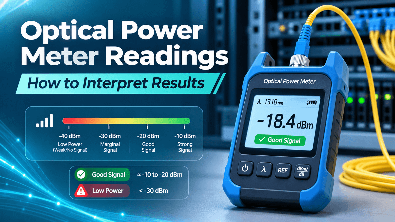
An optical power meter returns a precise number within seconds, yet that number can be read in several ways. The same display might show the strength of a live signal, the loss of a newly installed link, or a value distorted by a dirty connector or a mismatched setting.
Telling these cases apart is a routine part of fiber optic testing. The following article walks through what a reading represents, how to obtain results that can be compared, and how to turn them into a sound decision about the link.
What an Optical Power Meter Reading Means
A power meter reports the optical level arriving at its detector. Two questions shape how that value is read: which quantity it expresses, and under which conditions it was taken.
Distinguish Absolute Optical Power From Link Loss
The unit on the display identifies what kind of figure the meter is reporting. The difference between dBm and dB comes down to the reference point:
- dBm — absolute power relative to 1 milliwatt. 0 dBm equals 1 mW, and −10 dBm equals 0.1 mW.
- dB — a ratio between two power levels, used to express loss or gain. A change of 3 dB corresponds to roughly halving or doubling the signal.
A live receiver check produces an absolute value in dBm. A loss test compares the far-end level with a stored baseline and reports the difference in dB. Subtracting −18.4 dBm from a launch power of −5 dBm, for instance, gives 13.4 dB.
Because both scales are logarithmic, component losses in dB add directly. Three connections of 0.5 dB, 0.3 dB, and 0.75 dB contribute 1.55 dB in total.
Most optical power meters switch between both modes, so the selected unit needs to match the purpose of the test. Entering an absolute dBm value in a loss report would mix two unrelated figures.
Why Wavelength and Measurement Location Matter
Attenuation in the glass and detector response both vary with the optical band, so each result is valid for the band used during the measurement. Typical choices for fiber test wavelengths are:
- Multimode links — 850 nm and 1300 nm.
- Singlemode cabling — 1310 nm and 1550 nm, with 1625 nm added in some specifications.
The meter’s wavelength setting must match the source. A mismatch applies the wrong calibration factor and shifts the displayed value.
Location and direction add further context. Power measured at a receiver reflects the transmitter, the cabling, and any patch cords in that path. On duplex or bidirectional systems, each direction can show its own value.
This distinction separates two tasks:
- Operational received-power check — confirms that a live signal arrives within the receiver’s working range.
- Controlled insertion-loss test — uses a calibrated source and a stored baseline to measure the loss of the passive link itself.
How to Obtain a Comparable Measurement
A result can be compared with a requirement or an earlier session when the setup is clean, documented, and repeatable. Preparation begins at the end face, where small particles can shift a reading by tenths of a decibel or more.
Prepare Connectors and Check the Test Configuration
Connector contamination ranks among the most frequent causes of unexpected loss. Debris on one ferrule can also transfer to each mating surface it touches. A practical preparation sequence looks like this:
- Inspect each end face with a fiber microscope or video probe.
- Clean it with a suitable dry or wet-dry method if debris is visible.
- Inspect again and repeat cleaning until the end face passes.
- Connect promptly to avoid fresh contamination.
The sequence applies to the equipment side as well. Reference cords wear with repeated mating, so their end faces need regular inspection during a session.
Instrument settings call for a separate check. Confirm that connector types and polish (UPC or APC) are compatible and that the source has warmed up. Output drift after the baseline is set makes later readings unreliable.
For multimode links, the procedure may also call for a mode-control device such as a mandrel wrap. Launch conditions in the test cord affect the amount of attenuation the measurement shows.
Understand Reference Measurements for Insertion-Loss Tests
Fiber insertion loss is found by comparing the power through the link with a baseline captured before the link is added. That stored value is the reference measurement. A light source and a power meter used together for this purpose form an optical loss test set, and setting the baseline ties together four elements:
- A stable emitter at the specified wavelength.
- A power meter calibrated for the same band.
- Test reference cords of known quality that match the fiber type.
- A baseline-setting approach defined by the project’s procedure.
The selected method determines which mated pairs appear in the reported loss, depending on how many cords are used during referencing:
- One cord — the connections at both ends of the link are counted.
- Two cords — one of them is included.
- Three cords — both are left out, which suits cases where connector types or genders differ, as with some MPO systems.
Each approach yields its own value for the same link. The applicable test procedure should specify the method, and the report should state it.
Before testing begins, the reference cords can be verified by mating them and checking that the connection loss falls within the allowance stated for them.
Why Optical Power Readings Differ From Expectations
An unexpected value can originate in the link or in the test equipment. Checking both before reaching a conclusion reduces the risk of repairing cabling that works.
Investigate Loss and Instability in the Physical Link
High or fluctuating loss usually traces back to a small group of physical causes:
- Dirty or damaged end faces at patch panels and adapters.
- Tight bends or pinched cable.
- Poor fusion or mechanical splices.
- Mismatched fiber types, such as multimode cores of different sizes joined together.
- A worn adapter that lets the value shift when the cord moves.
Flexing the jumper gently while watching the display helps locate an intermittent connection. A visual fault locator can also reveal breaks or sharp bends near the test point by showing red light escaping from the fiber.
Comparing two wavelengths is another way to narrow the cause. Bending attenuates the longer band more strongly, so excess loss that appears mainly at 1550 nm often points to bending. A similar increase at 1310 nm and 1550 nm suggests a connector or splice.
Check Instrument Limitations Before Diagnosing a Fault
The meter and source have limits that can influence a result as strongly as the cabling. Before recording a fault, review the following:
- Measurement range — signals near the detector’s lower limit become noisy, and strong signals can exceed its upper limit.
- Display mode — a meter left in dB mode with an outdated baseline reports a relative figure that belongs to an earlier setup.
- Calibration status — both instruments are within their calibration interval.
- Uncertainty — one practical guideline places typical uncertainty at about ±10% of the measured loss, so a 2 dB result carries roughly ±0.2 dB.
- Adapter fit — the meter’s port adapter matches the cable plant.
A negative loss, where the link appears to add power, usually indicates a baseline set through a dirty or poorly mated connection. If the value changes after these checks, the original figure reflected the test setup.
How to Draw a Useful Conclusion From the Data
A verified result leads to a decision once it is compared with the correct benchmark and documented for later use.
Compare Against the Correct Power Budget or Loss Requirement
Fiber links are judged against two types of criteria, and each answers a separate question:
- Receiver power range — in a live system, received power has to fall between the receiver’s sensitivity and its overload level. The fiber optic link budget then subtracts expected losses from the transmitter’s minimum output to confirm that margin remains.
- Installation loss limit — for passive cabling, measured insertion loss is compared with an allowance calculated from cable length, connector pairs, and splices at the specified wavelength.
As an example, a transmitter with a minimum output of −3 dBm and a receiver sensitivity of −20 dBm leaves 17 dB for link losses and safety margin.
Both figures depend on system design and test method. A loss limit calculated for the one-cord approach applies to results obtained the same way. For this reason, acceptable dBm or dB values come from the equipment specifications and project documents for each link.
Record the Evidence and Choose Follow-Up Testing
A useful record lets another technician repeat the test and obtain a comparable result. It contains:
- Fiber or link ID and both end locations.
- Wavelength and, where relevant, transmission direction.
- Equipment models, serial numbers, and calibration dates.
- Reference method and reference value.
- Connector types and inspection results.
- Test date and measured value.
Records kept in a consistent structure also make it possible to trend a link across its service life.
Some questions call for a different tool. An OTDR shows where loss occurs along the fiber, which helps locate a faulty splice, bend, or break after excessive insertion loss has been found.
End-face inspection answers whether a specific connector is clean or damaged. For splice evaluation, OTDR traces taken from both ends and averaged give more dependable values, since a single direction can show apparent gains or exaggerated losses where dissimilar fibers are joined.
These methods add diagnostic detail. In most acceptance testing, the insertion-loss measurement remains the basis for comparing total link loss with its limit.
From Display Value to a Documented Fiber Decision
An optical power figure gains meaning through its context: the unit, the wavelength, the point of measurement, and, for loss tests, the reference method. Clean connectors and a matched, stable setup make the value comparable to requirements and earlier results.
When a reading looks unexpected, the practical sequence is to check the instruments and configuration first, then examine the physical link. A confirmed value is judged against the criterion that fits the test: a receiver power range for live systems or a calculated loss limit for installed cabling. A complete record of the conditions turns each measurement into evidence for acceptance, troubleshooting, and future comparison.